Overview

This tutorial gives a complete overview of MiTo’s core functionalities for mitochondrial single-cell lineage tracing (MT-scLT). The interested user is also encouraged to take a look at MiTo’s companion pipeline, nf-MiTo, which automates this data workflow at scale.

MiTo implements novel methods for MT-scLT (see our pre-print for motivation and estensive benchmarks). While optimized for scRNA-seq data (MAESTER protocol), MiTo can flexibly process data from other scLT systems (e.g., RedeeM, scWGS and Cas9-based lineage recorders).

This tutorial showcases the basic of MiTo APIs, which not only back up nf-MiTo lineage inference, but also enable interactive exploration of MT-scLT data straight after raw sequencing data pre-processing (see nf-MiTo documentation).

In particular, we will:

1. Load an AFM (AnnData format, output from nf-MiTo PREPROCESS)

2. Pre-process an AFM (i.e., cell and variant filtering, cell genotyping)

3. Compute pairwise cell-cell distances in the selected MT-SNV space

4. Infer mitochondrial cell phylogenies

5. Infer mitochondrial clones

On top of that, we will demonstrate how to use MiTo’s built-in metrics to evaluate the quality of our data and inferences, and provide examples on how to use MiTo’s powerful plotting library.

N.B: a properly configured MiTo environment is a necessary prerequisite for running this notebook. Follow the dedicated section of this documentation to install MiTo and its dependencies on your computing environment.

Dataset

This tutorial starts by downloding our test dataset from zenodo. Here, we will download the MDA_clones benchmarking dataset introduced in our recent pre-print. This is a tri-modal dataset including simoultaneous profiling of MT-SNVs, gene expression, and lentiviral barcodes (i.e., our ground truth clonal labels) for n=558 quality controlled cells.

# Set WD
WD='/Users/IEO5505/Desktop/MI_TO/MiTo/scratch'  # Change this to your working directory
!cd $WD

# Download and unzip test data
!wget https://zenodo.org/records/17225334/files/data_test.tar.gz && \
tar -xzvf data_test.tar.gz && \
rm data_test.tar.gz

--2025-10-01 16:29:44--  https://zenodo.org/records/17225334/files/data_test.tar.gz
Resolving zenodo.org (zenodo.org)... 188.185.48.194, 188.185.43.25, 188.185.45.92
Connecting to zenodo.org (zenodo.org)|188.185.48.194|:443... connected.
HTTP request sent, awaiting response... 200 OK
Length: 32419764 (31M) [application/octet-stream]
Saving to: ‘data_test.tar.gz’

data_test.tar.gz    100%[===================>]  30,92M  3,35MB/s    in 10s

2025-10-01 16:29:55 (3,07 MB/s) - ‘data_test.tar.gz’ saved [32419764/32419764]

x data_test/
x data_test/coverage.txt.gz
x data_test/cells_meta.csv
x data_test/afm_unfiltered.h5ad

The MDA_clones dataset we have just downloaded includes:

1. afm_unfiltered.h5ad: unfiltered AFM (the output from nf-MiTo PREPROCESS, with --pp_method = maegatk)

2. cells_meta.csv: cell metadata, including minimal QC covariates and ground truth clonal labels (GBC column)

3. coverage.txt.gz: cell-by-MT-genome-position coverage table

!ls data_test

afm_unfiltered.h5ad cells_meta.csv      coverage.txt.gz

Setup environment

We would also need to import all the necessary code, and to set up logging/visualization parameters:

import os
import logging
import numpy as np
import scanpy as sc
import mito as mt
import matplotlib.pyplot as plt
import plotting_utils as plu

# Logging
for handler in logging.root.handlers[:]:
    logging.root.removeHandler(handler)

logging.basicConfig(
    level=logging.INFO,
    format="%(asctime)s - %(levelname)s - %(message)s",
    force=True
)

# Plotting parameters
plu.set_rcParams({'figure.dpi':80})

# MiTo version and working directory
print(f"MiTo version: {mt.__version__}")
print(f"Working directory: {os.getcwd()}")

MiTo version: 0.0.9
Working directory: /Users/IEO5505/Desktop/MI_TO/MiTo/docs/source

Load the Allelic Frequency Matrix (AFM)

We can now load our unfiltered AFM:

afm = sc.read('data_test/afm_unfiltered.h5ad')
print(afm)
print(f'scLT system: {afm.uns["scLT_system"]}')
print(f'Pre-processing pipeline adopted: {afm.uns["pp_method"]}')
print(f'Raw basecalls metrics: {afm.uns["raw_basecalls_metrics"]}')

AnnData object with n_obs × n_vars = 558 × 18846
    obs: 'GBC', 'sample', 'nUMIs', 'mito_perc', 'detected_genes', 'cell_complexity', 'doublet_score', 'predicted_doublet', 'passing_mt', 'passing_nUMIs', 'passing_ngenes', 'n_genes', 'mean_site_coverage', 'median_target_site_coverage', 'median_untarget_site_coverage', 'frac_target_site_covered'
    var: 'pos', 'ref', 'alt'
    uns: 'pp_method', 'raw_basecalls_metrics', 'scLT_system'
    layers: 'AD', 'DP', 'qual', 'site_coverage'
scLT system: MAESTER
Pre-processing pipeline adopted: maegatk
Raw basecalls metrics: {'total_basecalls': 6559093, 'variant_basecalls': 192201, 'variant_basecalls_for_annot_cells': 192201}

As we can see, our afm is an AnnData object equipped with the following slots:

• .obs: cell metadata, with minimal QC covariates and ground truth clonal labels (i.e., GBC column) from lentiviral barcoding

• .var: variant (MT-SNVs) metadata (minimal MT-SNVs annotation is present in this unfiltered AFM, but it will be updated in the next pre-processing steps)

• .uns: dataset parameters (e.g., pp_method and scLT_system) and metrics (e.g., raw_basecalls_metrics)

• .layers: 4 parallel cell x variant site sparse matrices

At this stage, this afm.layers include:

• AD: alternative allele total UMI counts

• DP: total UMI counts (DP can be >0 only for entries with AD>0)

• qual: average base calling quality

• site_coverage: total UMI counts (site_coverage can be >0 even for entries with AD=0)

Our .X slot instead store “raw” Allelic Frequencies (AFs, i.e., AD / site coverage).

# Selection of cells (n=2, rows) and variants (n=3, columns) with most non-zero AF values
cells = (afm.X>0).sum(axis=1).A1.argsort()[::-1][:2]
variants = (afm.X>0).sum(axis=0).A1.argsort()[::-1][:3]

# Print out each layer subsection
print('AF')
print(afm[cells, variants].X.toarray())
print('AD')
print(afm[cells, variants].layers['AD'].toarray())
print('DP')
print(afm[cells, variants].layers['DP'].toarray())
print('qual')
print(afm[cells, variants].layers['qual'].toarray())
print('site_coverage')
print(afm[cells, variants].layers['site_coverage'].toarray())

AF
[[1.        0.9994376 1.       ]
 [1.        1.        1.       ]]
AD
[[3043 1777 1859]
 [2962 1446 2492]]
DP
[[3043 1778 1859]
 [2962 1446 2492]]
qual
[[45 45 45]
 [45 45 45]]
site_coverage
[[3043. 1778. 1859.]
 [2962. 1446. 2492.]]

We can now proceed with AFM pre-processing.

AFM pre-processing

Proper AFM pre-processing is crucial for robust lineage inference (see our pre-print), and MiTo provides highly-optimized methods to handle this important analysis step.

Cell Filtering

As mentioned, cells in the unfiltered AFM have already passed standard Gene Expression QC. However, we still need make sure that only cells with an high-quality MT-SNVs profile are included in downstream analysis. Specifically, here we are looking for cells with sufficiently high and evenly distributed coverage across the entire MT-genome (or MAESTER target sites, ~13k sites across the ~16kB MT-genome). To perform cell filtering, MiTo implements the mt.pp.filter_cells function:

afm = mt.pp.filter_cells(afm, cell_filter='filter2')
afm_raw = afm.copy()  # Keep a copy of the AFM with all MT-SNVs, for visualization purposes

2025-10-01 17:37:51,988 - INFO - scLT system: MAESTER
2025-10-01 17:37:52,042 - INFO - Filtered cells (i.e., median target MT-genome coverage >=25 and fraction covered sites >=0.75: 375

As we can see, the number of cells dropped from 558 to 375 (i.e., 37% of the starting cells were filtered out because they did not satisfy the necessary quality standards).

MT-SNVs filtering

We can now proceed with next step: MT-SNVs filtering. To do this, we will use the mt.pp.filter_afm function:

afm = mt.pp.filter_afm(afm, filtering='MiTo')

2025-10-01 17:37:54,487 - INFO - Compute general dataset metrics...
2025-10-01 17:37:54,489 - INFO - Compute vars_df as in Weng et al., 2024
2025-10-01 17:37:54,826 - INFO - Filter MT-SNVs...
2025-10-01 17:37:54,827 - INFO - scLT_system: MAESTER
2025-10-01 17:37:54,827 - INFO - pp_method: maegatk
2025-10-01 17:37:54,827 - INFO - Feature selection method: MiTo
2025-10-01 17:37:54,827 - INFO - Original afm: n cells=375, n features=18494
2025-10-01 17:37:54,941 - INFO - afm after baseline filter: n cells=375, n features=4366
2025-10-01 17:37:54,941 - INFO - Re-annotate variants in afm
2025-10-01 17:37:55,023 - INFO - afm after MiTo filter: n cells=375, n features=34
2025-10-01 17:37:55,026 - INFO - Exclude 1 common SNVs events (dbSNP)
2025-10-01 17:37:55,048 - INFO - Exclude 0 common RNA editing events (REDIdb)
2025-10-01 17:37:55,059 - INFO - Assign MT-genotypes with MiTo method
2025-10-01 17:37:55,539 - INFO - n MT-SNVs genotyped with binomial mixtures: 10
2025-10-01 17:37:55,542 - INFO - Retain only cells with at least 1 MT-SNVs: 372
2025-10-01 17:37:55,545 - INFO - Remove MT-SNVs with no +cells having at least 2 AD counts
2025-10-01 17:37:55,546 - INFO - Use precomputed bin layer: bin_method=MiTo, binarization_kwargs={'t_prob': 0.7, 't_vanilla': 0.0, 'min_AD': 2, 'min_cell_prevalence': 0.1}
2025-10-01 17:37:55,547 - INFO - Compute distances: ncores=8, metric=weighted_jaccard.
2025-10-01 17:37:55,554 - INFO - Filter only MT-SNVs with significant spatial auto-correlation (i.e., Moran I statistics)
2025-10-01 17:37:55,690 - INFO - Re-annotate variants in afm
2025-10-01 17:37:55,694 - INFO - Retain cells with at least 1 MT-SNVs: 288
2025-10-01 17:37:55,694 - INFO - Final afm after all filters: n cells=288, n features=24
2025-10-01 17:37:55,694 - INFO - Compute last (filtered) statistics.

As we can see from the printed logs, mt.pp.filter_afm performs different tasks to ensure only high-quality MT-SNVs (and the respective variant-bearing cells) are included for lineage inference (see our pre-print Supplementary Methods).

print(afm)

AnnData object with n_obs × n_vars = 288 × 24
    obs: 'GBC', 'sample', 'nUMIs', 'mito_perc', 'detected_genes', 'cell_complexity', 'doublet_score', 'predicted_doublet', 'passing_mt', 'passing_nUMIs', 'passing_ngenes', 'n_genes', 'mean_site_coverage', 'median_target_site_coverage', 'median_untarget_site_coverage', 'frac_target_site_covered'
    var: 'pos', 'ref', 'alt', 'mean_af', 'mean_cov', 'quality', 'n0', 'n1', 'n2', 'n5', 'n10', 'n50', 'Variant_CellN', 'median_af_in_positives', 'mean_AD_in_positives', 'mean_DP_in_positives'
    uns: 'pp_method', 'raw_basecalls_metrics', 'scLT_system', 'cell_filter', 'dataset_metrics', 'genotyping', 'distance_calculations', 'char_filter'
    layers: 'AD', 'DP', 'qual', 'site_coverage', 'bin'
    obsp: 'distances'

Our final pre-processed AFM include 288 high-quality cells and 24 MT-SNVs. As shown, mt.pp.filter_afm internally calls mt.pp.call_genotypes and mt.pp.compute_distances, which assign binary genotypes to each cell/MT-SNV combination (the new bin layer in afm.layers) and compute cell-cell distances in this binarized feature space (with the default weighted_jaccard distance metric, see the new distances slot in afm.obsp). mt.pp.filter_afm also annotates variants (afm.var) and update AFM parameters and metrics in afm.uns.

Dimensionality reduction

Cell-cell distances can be used together with feature matrices to reduce the dimensionality of the dataset and visualize relevent patterns in the data. MiTo’s mt.pp.reduce_dimensions performs this operation:

mt.pp.reduce_dimensions(afm, method='UMAP')
print(afm)

2025-10-01 17:38:26,222 - INFO - Use bin layer
2025-10-01 17:38:26,223 - INFO - Use precomputed distances

AnnData object with n_obs × n_vars = 288 × 24
    obs: 'GBC', 'sample', 'nUMIs', 'mito_perc', 'detected_genes', 'cell_complexity', 'doublet_score', 'predicted_doublet', 'passing_mt', 'passing_nUMIs', 'passing_ngenes', 'n_genes', 'mean_site_coverage', 'median_target_site_coverage', 'median_untarget_site_coverage', 'frac_target_site_covered'
    var: 'pos', 'ref', 'alt', 'mean_af', 'mean_cov', 'quality', 'n0', 'n1', 'n2', 'n5', 'n10', 'n50', 'Variant_CellN', 'median_af_in_positives', 'mean_AD_in_positives', 'mean_DP_in_positives'
    uns: 'pp_method', 'raw_basecalls_metrics', 'scLT_system', 'cell_filter', 'dataset_metrics', 'genotyping', 'distance_calculations', 'char_filter'
    obsm: 'X_umap'
    layers: 'AD', 'DP', 'qual', 'site_coverage', 'bin'
    obsp: 'distances'

In this case, the default UMAP method is used to embed cells in a 2-dimensional space stored as the new X_umap entry in the .obsm slot of our AFM. We will visualize these embeddings later.

(Optional) Filtered MT-SNVs space quality assessment

Pre-processing of our AFM is now done!

Since this dataset comes with ground truth clonal labels, we can optionally check the quality of our MT-SNV space and its associated cell-cell distances. To do so, we first compute a k-nearest neighbor (kNN) graph of our cells (mt.pp.kNN_graph function), and then we use metrics that evaluate how well cell-cell distances can separate ground truth clonal populations (i.e., the categorical labels in the GBC column of afm.obs).

# Extract distance matrix and compute k-NN graph
D = afm.obsp['distances'].toarray()
idx, _, _ = mt.pp.kNN_graph(D=D, k=15, from_distances=True)

# Compute lineage quality metrics using ground truth GBC labels
auprc = mt.ut.distance_AUPRC(D, afm.obs['GBC'])
kbet_score = mt.ut.kbet(idx, afm.obs['GBC'])
nn_entropy = mt.ut.NN_entropy(idx, afm.obs['GBC'])
nn_purity = mt.ut.NN_purity(idx, afm.obs['GBC'])

# Print out metrics
print(f"- Distance AUPRC: {auprc:.3f}")
print(f"- kBET score: {kbet_score:.3f}")
print(f"- NN entropy: {nn_entropy:.3f}")
print(f"- NN purity: {nn_purity:.3f}")

- Distance AUPRC: 0.778
- kBET score: 0.483
- NN entropy: 1.078
- NN purity: 0.571

For details on these metrics choice and motivation, refer to our pre-print Supplementary Methods.

Lineage inference

After AFM pre-processing, lineage inference can start. First we will infer a mitochondrial cell phylogeny, and then, we will use this phylogeny to infer discrete mitochondrial clones.

Mitochondrial phylogenies

Phylogeny inference first, then. To accomplish this, we use the mt.tl.build_tree function, which implements several solvers from the cassiopeia package. Here, we use the the Unweighted Pair Group Method with Arithmetic Mean (UPGMA) method. Note that, on top of cassiopeia solvers, nf-MiTo support other tree-building algorithms (i.e., mpboot and iqtree, see nf-MiTo for reference).

tree = mt.tl.build_tree(afm, precomputed=True, solver='UPMGA')

2025-10-01 17:38:48,213 - INFO - Use precomputed distances: metric=weighted_jaccard, layer=bin
2025-10-01 17:38:48,214 - INFO - Precomputed bin layer: bin_method=MiTo and binarization_kwargs={'t_prob': 0.7, 't_vanilla': 0.0, 'min_AD': 2, 'min_cell_prevalence': 0.1}
2025-10-01 17:38:48,217 - INFO - Build tree: metric=weighted_jaccard, solver=UPMGA

Mitochondrial clones

We can now use this mitochondrial phylogeny to infer discrete clonal labels. For this, we will use the mt.tl.MiToTreeAnnotator class and its clonal_inference method.

model = mt.tl.MiToTreeAnnotator(tree)
model.clonal_inference()

2025-10-01 17:38:52,657 - INFO - Retrieve cell assignment to tree clades
2025-10-01 17:38:52,691 - INFO - Compute mutations enrichment
2025-10-01 17:38:53,449 - INFO - Start Grid Search. n hyper-parameter combinations to explore: 36
Grid Search: 100%|██████████| 36/36 [00:09<00:00,  3.87it/s]
2025-10-01 17:39:02,745 - INFO - Hyper-params chosen: similarity_percentile=90, mut_enrichment_treshold=3, merging_treshold=0.5
2025-10-01 17:39:02,975 - INFO - Compute expansion pvalues
2025-10-01 17:39:02,977 - INFO - Estimate cell fitness scores

node_ranking: inferring ancestral fitness... done in  1.71 s
node_ranking: calculating alternative rankings... done in  0.11 s

2025-10-01 17:39:06,636 - INFO - MiTo clonal inference finished. 13.98 s

(Optional) lineage inference evaluation

Evaluate the quality of our lineage inference using metrics that evaluate the correlation between tree topology and underlying character distances, the evolutionary pattern of MT-SNVs on tree branches, and the relationship between ground truth clones (GBC) and MiTo clones:

# Tree structure metrics
corr_distances, _ = mt.ut.calculate_corr_distances(tree)
ci_scores = mt.ut.CI(tree)
ri_scores = mt.ut.RI(tree)

print(f"Tree-structure metrics:")
print(f"- Distances correlation: {corr_distances:.3f}")
print(f"- Median CI: {np.median(ci_scores):.3f}")
print(f"- Median RI: {np.median(ri_scores):.3f}")

# Clonal assignment metrics
test_mask = tree.cell_meta['MiTo clone'].isna()
assigned_cells = ~test_mask
gbc_assigned = tree.cell_meta.loc[assigned_cells, 'GBC']
mito_assigned = tree.cell_meta.loc[assigned_cells, 'MiTo clone']
ari = mt.ut.custom_ARI(gbc_assigned, mito_assigned)
nmi = mt.ut.normalized_mutual_info_score(gbc_assigned, mito_assigned)

print(f"Clonal assignment metrics:")
print(f"- Adjusted Rand Index: {ari:.3f}")
print(f"- Normalized Mutual Information: {nmi:.3f}")

Tree-structure metrics:
- Distances correlation: 0.595
- Median CI: 0.292
- Median RI: 0.996
Clonal assignment metrics:
- Adjusted Rand Index: 0.950
- Normalized Mutual Information: 0.928

For more details on these metrics, please refer to our pre-print Supplementary Methods.

Visualization

We have pre-processed our AFM and leverage MT-SNVs to infer mitochondrial cell lineages. We can now create comprehensive visualizations to assess our results.

MT-SNVs selection

First, we would like to visualize the properties of our filtered MT-SNVs callset.

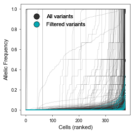
We start by plotting the Allelic Frequency spectrum of MT-SNVs before and after AFM pre-processing:

# Annotate vars in afm_raw
mt.pp.annotate_vars(afm_raw)

# Set colors
colors = {'All variants': '#303030', 'Filtered variants': '#05A8B3'}

# Plot allele frequency spectrum (before vs after filtering)
fig, ax = plt.subplots(figsize=(3.5,3.5))
mt.pl.vars_AF_spectrum(afm_raw, ax=ax, color=colors['All variants'], alpha=.7, linewidth=.2)
mt.pl.vars_AF_spectrum(afm_raw[:,afm.var_names], ax=ax, color=colors['Filtered variants'], linewidth=.5, alpha=1)
plu.add_legend(colors, ax=ax, loc='upper left', bbox_to_anchor=(0.05,.95), frameon=False)
fig.tight_layout()
plt.show()

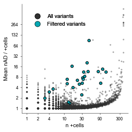
We would also like to visualize the number of positive cells (+cells) vs the average number of UMIs supporting alternative allele basecalls across +cells, for each MT-SNV:

# Set xticks
xticks = [1, 2, 4, 10, 30, 90, 300, 1100]

# Plot number of cells vs mean alternative allele depth
fig, ax = plt.subplots(figsize=(3.5,3.5))
mt.pl.plot_ncells_nAD(afm_raw, ax=ax, xticks=xticks, color='#303030', s=2, alpha=.3, label='All variants')
mt.pl.plot_ncells_nAD(afm, ax=ax, color='#05A8B3', xticks=xticks, s=5, alpha=1, markeredgecolor='k', label='Filtered variants')
plu.format_ax(ax=ax, ylabel='Mean nAD / +cells', xlabel='n +cells', reduced_spines=True)
plu.add_legend(colors, ax=ax, loc='upper left', bbox_to_anchor=(0.05,.95), frameon=False)
fig.tight_layout()
plt.show()

2025-10-01 17:58:11,383 - INFO - Re-annotate variants in afm
2025-10-01 17:58:11,798 - INFO - Re-annotate variants in afm

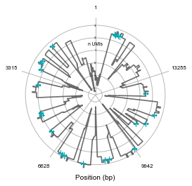
We might also want to know where are these MT-SNVs distributed across the MT-genome

# Load coverage data
cov = mt.io.read_coverage(afm_raw, 'data_test/coverage.txt.gz', 'MDA_clones')

# Visualize MT genome coverage in polar coordinates, with MT-SNVs highlighted
fig, ax = plt.subplots(figsize=(3.5,3.5), subplot_kw={'projection': 'polar'})
mt.pl.MT_coverage_polar(
    cov,
    var_subset=afm.var_names, ax=ax,
    yticks_size=4,
    kwargs_subset={'markersize': 8, 'c': '#05A8B3', 'label': 'Selected variants'},
    kwargs_main={'c': '#303030', 'linewidth': 1.5, 'alpha': .7, 'label': 'All positions'}
)
fig.tight_layout()
plt.show()

24

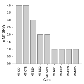
… which MT-gene harbour them

# Load MT-genes annotation
ref_df = mt.ut.load_mt_gene_annot()
df_plot = ref_df.query('mut in @afm.var_names')

# Plot variant distribution across MT genes
fig, ax = plt.subplots(figsize=(3.5,3.5))
plu.counts_plot(df_plot, 'Symbol', width=.8, ax=ax, color='#C0C0C0', edgecolor='k', with_label=False)
plu.format_ax(ax=ax, rotx=90, ylabel='n MT-SNVs', xlabel='Gene', reduced_spines=True)
fig.tight_layout()
plt.show()

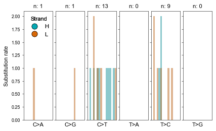
… and which mutational signatures are they enriched for:

fig = mt.pl.mut_profile(afm.var_names, figsize=(6,3.5))
fig.tight_layout()
plt.show()

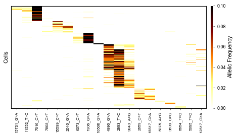
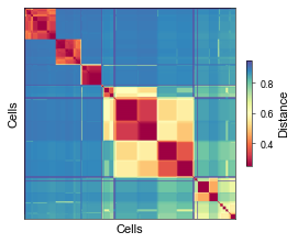
We would also like to visualize our characters and cell-cell distances in clustered heatmaps:

fig, ax = plt.subplots(figsize=(6,3.5))
mt.pl.heatmap_variants(afm, ax=ax, cmap='afmhot_r')
fig.tight_layout()
plt.show()

2025-10-01 17:59:40,480 - INFO - Compute tree from precomputed cell-cell distances...
2025-10-01 17:59:40,481 - INFO - Use precomputed distances: metric=weighted_jaccard, layer=bin
2025-10-01 17:59:40,482 - INFO - Precomputed bin layer: bin_method=MiTo and binarization_kwargs={'t_prob': 0.7, 't_vanilla': 0.0, 'min_AD': 2, 'min_cell_prevalence': 0.1}
2025-10-01 17:59:40,483 - INFO - Build tree: metric=weighted_jaccard, solver=UPMGA
2025-10-01 17:59:40,613 - INFO - Retrieve cell assignment to tree clades
2025-10-01 17:59:40,626 - INFO - Compute mutations enrichment

fig, ax = plt.subplots(figsize=(3.5, 3.5))
mt.pl.heatmap_distances(afm, ax=ax, cmap='Spectral')
fig.tight_layout()
plt.show()

2025-10-01 18:06:04,930 - INFO - Compute tree from precomputed cell-cell distances...
2025-10-01 18:06:04,931 - INFO - Use precomputed distances: metric=weighted_jaccard, layer=bin
2025-10-01 18:06:04,932 - INFO - Precomputed bin layer: bin_method=MiTo and binarization_kwargs={'t_prob': 0.7, 't_vanilla': 0.0, 'min_AD': 2, 'min_cell_prevalence': 0.1}
2025-10-01 18:06:04,935 - INFO - Build tree: metric=weighted_jaccard, solver=UPMGA

Lineage inference

Before dealing with phylogeny inference diagnostics, we would also like to visualize if our ground-truth labels cluster in UMAP space.

fig, ax = plt.subplots(figsize=(5, 3.5))
colors = plu.create_palette(afm.obs, 'GBC', sc.pl.palettes.vega_10_scanpy)
mt.pl.draw_embedding(afm, feature='GBC', ax=ax, categorical_cmap=colors, legend=True, size=150)
plt.subplots_adjust(right=.7)
plt.show()

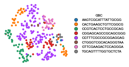
As we can see, to a great extent, lentiviral clones nicely cluster together.

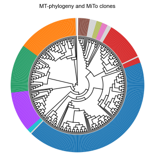
Finally we would like to visualize our main downstream analysis product, our cell phylogeny and MiTo clones:

fig, ax = plt.subplots(figsize=(4, 4.2))
mt.pl.plot_tree(tree, ax=ax, features=['MiTo clone'], colorstrip_width=7.5)
ax.set_title('MT-phylogeny and MiTo clones')
fig.tight_layout()
plt.show()

Summary

🎉 Congratulations! You’ve successfully gone through the basics of MiTo!

Outlook

More detailed tutorials starting from the nf-MiTo INFER output (bootstrapped cell phylogenies), will be soon available.